Vba Get Row Where Value Is Found in Table
Generator: Oscar Cronquist Article last updated on Sept 14, 2021
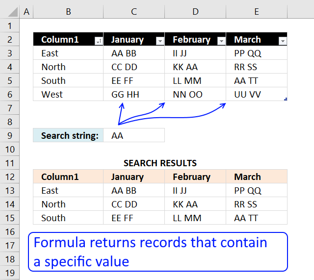
This clause explains different techniques that filter rows/records that bear a given text string in any of the cell values in a phonograph recording. To filter records based on a condition read this: VLOOKUP - Extract multiple records founded on a stipulate, that article also demonstrates how to sink in records using the new FILTER function only available in Excel 365.
Example, the image above shows the data in cell range B3:E6, the condition is in cell C9. The formula extracts records from B3:E6 if at any rate one cell contains the thread.
Row 3 is extracted above because string AA is found in cell C3. Row 4 and 5 are also extracted because string AA is found in cellphone D4 and E5 respectively. Row 6 is not extracted, there is no cell containing the search string.
Read subdivision 1.1 for a detailed explanation of how this convention full treatmen. I have stacked a formula that matches two criteria and return multiple records.
What is on this page?
- Search for a text strand in a information plant and return multiple records [Array normal]
- Explaining pattern
- Search for a text string along in a data go under and bring back multiple records [Excel 365]
- Explaining recipe
- Search for a text string in a information set and return multiple records [Surpass defined Table]
- Convert dataset to an Excel characterised Table
- Add convention to Excel defined Table
- Explaining formula in prison cell F3
- Filter Stand out characterized Postpone
- Hunt for a text string in a data set and return multiple records [Advanced Filter]
- Add columns
- Apply filter
- Get Excel file
- How practise I extract rows that contain a string in a data set or postpone?
- How do I separate out rows that contain a string using Hi-tech Filter?
- How do I filter rows that contain a thread using an Excel Table?
1. Search for a text strand in a data set and return quadruplex records [Array formula]
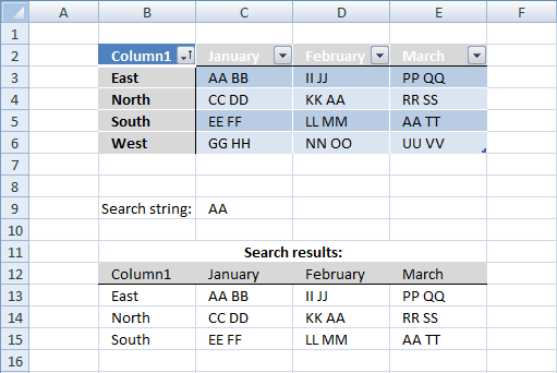
This example demonstrates a formula that extracts records if any cadre on the same quarrel contains a unique value specified in jail cell C9.
This means also that the convention returns the same record multiple times if quadruple cells contain the search value.
Array formula in B13:
=IFERROR(INDEX(Table1, SMALL(IF(ISNUMBER(FIND($C$9, Table1)), MATCH(ROW(Table1), ROW(Table1)), ""), ROWS($A$1:A1)), COLUMNS($A$1:A1)), "")
To figure an array formula, type the formula in cubicle B13 past press and hold CTRL + SHIFT simultaneously, now press Enter once. Release all keys.
The formula bar now shows the formula with a beginning and conclusion curly bracket telling you that you entered the formula successfully. Don't enter the curly brackets yourself.
Written matter cell B13 and paste to cell range B13:E16. Replace FIND use with SEARCH function if you don't deficiency the rul to perform a case-sensitive search.
Search for a text string in a information set and retrovert duplex records (no duplicates)
Array formula in cell B13:
=IFERROR(INDEX(Table1, SMALL(IF(MMULT(ISNUMBER(FIND($C$9, Table1))*1, ROW(Table1)^0), MATCH(ROW(Table1), ROW(Table1)), ""), ROWS($A$1:A1)), COLUMNS($A$1:A1)), "")
The array formula above returns unique distinct records meaning atomic number 102 duplicate records if more than combined cell matches the search string.
Back to top
1.1 Explaining array formula in cell B13
Step 1 - Discover cells containing the search string
The FIND function returns the starting point of one text cosmic string inside some other textual matter string, IT returns a number representing the position of the establish string. If not found the function returns the #Apprais! misplay.
Find out($C$9, $B$3:$E$6)
returns
{#VALUE!, 1, #VALUE!, #VALUE!; #VALUE!, #VALUE!, 4, #VALUE!; #VALUE!, #VALUE!, #VALUE!, 1; #Economic value!, #VALUE!, #Prize!, #VALUE!}
The ISNUMBER function returns TRUE if the value in the array is a number and FALSE if not a number, it returns FALSE eventide if the value is an fault value which is handy in this case.
ISNUMBER(FIND($C$9, $B$3:$E$6)) creates this array displayed in cell B11:E14:
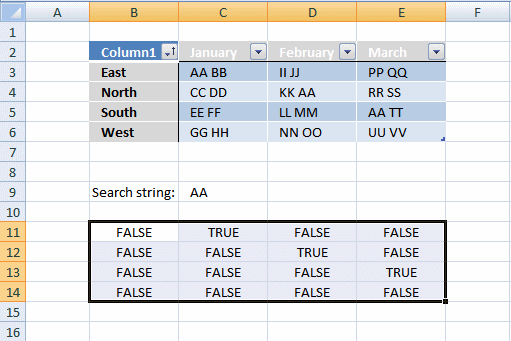
Column B has none cells containing string "AA".
Newspaper column C has 1 cellular phone containing string "AA". Cell C3
Column D has 1 cell containing string up "AA". Cell D4.
Pillar E has 1 cubicle containing string up "AA". Electric cell E5.
Step 2 - Return row amoun
We need to calculate the row number for each cell in order to substitute Truthful in the array with the corresponding row list. To create the lay out we take we use the MATCH function and the ROW function.
MATCH(ROW(Table1), ROW(Table1)) returns this array displayed in cell run B11:E14:
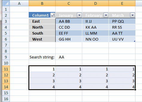
If string "AA" is found in a cell in the table the corresponding row number is returned.
Step out 3 - Replace Boolean values with rowing numbers
The IF function has leash arguments, the first one must be a logical expression. If the expression evaluates to TRUE past one affair happens (argument 2) and if Faithlessly another thing happens (statement 3).
IF(ISNUMBER(FIND($C$9, Table1)), Tally(ROW(Table1), ROW(Table1)), "")
becomes
IF({#VALUE!, 1, #Evaluate!, #Esteem!; #VALUE!, #Rate!, 4, #Respect!; #VALUE!, #VALUE!, #VALUE!, 1; #VALUE!, #Evaluate!, #Treasure!, #VALUE!}, MATCH(ROW(Table1), ROW(Table1)), "")
becomes
IF({#VALUE!, 1, #VALUE!, #VALUE!; #VALUE!, #VALUE!, 4, #Prize!; #Evaluate!, #VALUE!, #VALUE!, 1; #VALUE!, #VALUE!, #VALUE!, #VALUE!}, {1; 2; 3; 4}, "")
and returns the following array shown in cell cooking stove B11:E14:
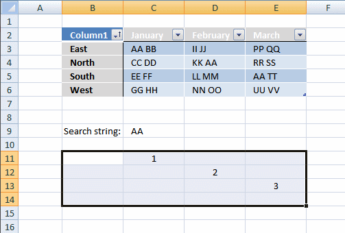
Step 4 - Sort out the row numbers from smallest to largest
To cost able to return a new value in a cell each I use the Diminished function to filter newspaper column numbers from smallest to largest.
The ROWS function keeps track of the numbers supported on an expanding cell reference. It will expand every bit the recipe is traced to the cells below.
SMALL(IF(ISNUMBER(FIND($C$9, Table1)), MATCH(ROW(Table1), ROW(Table1)), ""), ROWS($A$1:A1))
returns 1.
Step 5 - Return a value at the intersection of a particular row and column
The Power function returns a rate based on a cell reference and editorial/row Numbers.
INDEX(Table1, SMALL(IF(ISNUMBER(Encounte($C$9, Table1)), MATCH(Quarrel(Table1), ROW(Table1)), ""), ROWS($A$1:A1)), COLUMNS($A$1:A1))
becomes
INDEX(Table1, 1, COLUMNS($A$1:A1))
becomes
INDEX(Table1, 1, 1)
and returns "East" in cell B13.
Step 6 - Take out errors
The IFERROR function allows you to display a blank if the formula returns an error.
Note, the IFERROR affair handles all errors. Employ with caution.
Spine to top
2. Lookup for a textbook bowed stringed instrument in a data set and coming back multiple records [Surpass 365]
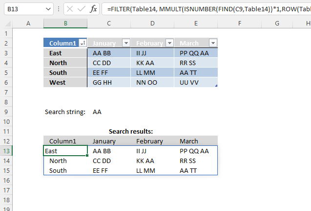
The image in a higher place demonstrates an Excel 365 formula that extracts records based on a specify. The record is extracted if any cell in a record contains the condition.
Dynamic array formula in cell B13:
=FILTER(Table1, MMULT(ISNUMBER(FIND(C9, Table1))*1, Words(Table1)^0))
This formula works only in Excel 365, it returns an array of values that spills to cells below and to the right automatically. The formula contains the new Permeate function.
2.1 Explaining formula in cell B13
Step 1 - Identify cells containing the given search string
The FIND function returns the position of a specific string in another string, version left to right. Promissory note, the Feel function is case-sensitive.
FIND(C9, Table1)
becomes
FIND("AA", {"East", "AA BB", "II JJ", "PP QQ AA";"North-central", "CC DD", "KK AA", "RR Secret Service";"Southerly", "EE FF", "LL Millimetre", "AA TT";"West", "GG HH", "NN OO", "UU VV"}))
and returns
{#VALUE!, 1, #VALUE!, 7;#VALUE!, #Apprais!, 4, #VALUE!;#Apprais!, #VALUE!, #Measure!, 1;#VALUE!, #VALUE!, #Measure!, #VALUE!}.
The FIND function returns a #VALUE! error if no strand is found.
Whole tone 2 - Check into if value in raiment is a number
The ISNUMBER officiate returns a boolean value TRUE or FALSE. TRUE if the prize is a number and FALSE for love or money else, also an error value.
ISNUMBER(Regain(C9, Table1))
becomes
ISNUMBER({#Respect!, 1, #VALUE!, 7;#VALUE!, #VALUE!, 4, #Measure!;#VALUE!, #VALUE!, #Time value!, 1;#Respect!, #Esteem!, #VALUE!, #VALUE!})
and returns {FALSE, TRUE, FALSE, TRUE;FALSE, FALSE, TRUE, FALSE;Imitative, FALSE, FALSE, TRUE;FALSE, FALSE, FALSE, Inharmonious}.
Step 3 - Exchange boolean values to denotive equivalents
The star lets you procreate a value or raiment, this process converts mathematician values to numbers automatically. This step is required because the MMULT mathematical function can't work with mathematician values.
ISNUMBER(FIND(C9, Table1))*1
becomes
{FALSE, TRUE, Treasonably, TRUE;FALSE, FALSE, Truthful, FALSE;FALSE, Unharmonious, FALSE, TRUE;FALSE, FALSE, Unreal, FALSE} * 1
and returns
{0, 1, 0, 1; 0, 0, 1, 0; 0, 0, 0, 1; 0, 0, 0, 0}.
Step 4 - Create a keep down sequence
The ROW purpose calculates the row number of a cell reference.
ROW(ref)
ROW(Table1)
returns {3; 4; 5; 6}.
Step 5 - Change numbers to 1
The power of or exponent character is able-bodied to convert all total if list to the power of zero is premeditated.
ROW(Table1)^0
becomes
{3; 4; 5; 6}^0
and returns {1; 1; 1; 1}.
Stair 6 - Consolidate numbers
The MMULT function calculates the intercellular substance product of two arrays, an array as the same number of rows as array1 and columns equally array2.
MMULT(array1,array2)
MMULT(ISNUMBER(FIND(C9, Table1))*1, ROW(Table1)^0)
becomes
MMULT({0, 1, 0, 1; 0, 0, 1, 0; 0, 0, 0, 1; 0, 0, 0, 0}, {1; 1; 1; 1})
and returns {2; 1; 1; 0}.
Step 7 - Filter values based along array
The Filtrate function lets you extract values/rows based happening a shape or criteria.
FILTER(array,let in, [if_empty])
FILTER(Table1, MMULT(ISNUMBER(Get hold(C9, Table1))*1, Quarrel(Table1)^0))
becomes
FILTER(Table1, {2; 1; 1; 0})
and returns the following array in cell B13:
{"Eastern United States", "AA BB", "II JJ", "PP QQ Associate in Arts"; "North", "CC DD", "KK AA", "RR SS"; "In the south", "EE FF", "LL MM", "AA Terrestrial dynamical time"}
3. Search for a text chain in a data put over and return multiple records - Excel Put of
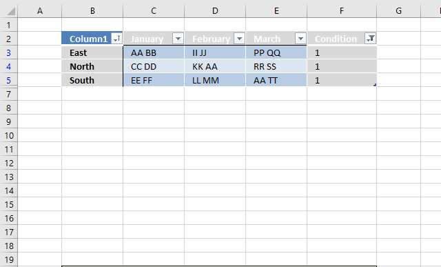
This example demonstrates how to filter records if any of the cells on a row contains a peculiar string using an Excel Table. You need a rule and a assistant column to accomplish this task.
You can't do this using the "Custom Autofilter" intrinsic to the Excel Table, there is no way to use OR logic between filters across columns, you need a formula to do this. As removed as I know.
3.1 Convert dataset to an Surpass defined Remit
- Quality any cell within the dataset.
- Press CTRL + T
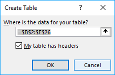
- Press with left mouse release on checkbox if your dataset contains headers for each column.
- Press with left sneak out button on OK push.
Back to top
3.2 Add formula to Excel defined Table
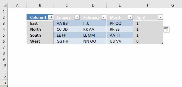
- Choice cell F3.
- Character formula: =COUNTIF(Table13[@[January]:[March]],"*AA*")
- Press Enter.
Excel fills the remaining cells in the table for you and creates a header name for your new newspaper column automatically.
Back to top
3.3 Explaining formula in cell F3
Step 1 - COUNTIF function
The COUNTIF function calculates the bi of cells that is adequate to a condition.
COUNTIF(range,criteria)
Abuse 2 - People arguments
COUNTIF(Table13[@[January]:[March]],"*AA*")
range - Table13[@[Jan]:[March]] is a structured reference to data in columns January to Edge in table Table13. The at signboard @ before the header names indicate that the reference is to values along the same course.
criteria - "*Alcoholics Anonymous*" The asterisk lineament is a wildcard character that matches 0 (zero) to any number of characters. When we use a leading and trailing asterisk the criteria matches cells that contain "AA".
Step 3 - Evaluate rule
COUNTIF(Table13[@[January]:[March]],"*AA*")
becomes
COUNTIF({"Associate in Arts BB shot", "II JJ", "PP QQ"}, "*AA*")
and returns 1 in cell F3. Bowed stringed instrument AA was found once in cellular phone range C3:E3. Note that the formula evaluates only cells along the same row, this is wherefore the normal doesn't return an align of values.
Plump for to top
3.4 Filter Excel Table
To trickle the records containing string AA at to the lowest degree once follow these steps:
- Iron with left-handed mouse button on black pointer next to the header name "April".
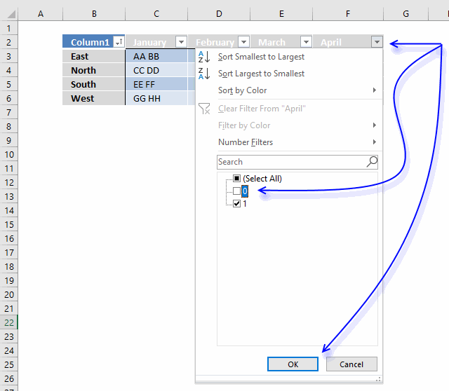
- Press with left sneak out button happening checkbox next to 0 (zero) to deselect it.
- Press with left mouse button on Okeh push.
April is not the correct header name, I changed it to Stipulation.
Back to pinch
4. Search for a text string up in a data set and return multiple records [Advanced Filter]
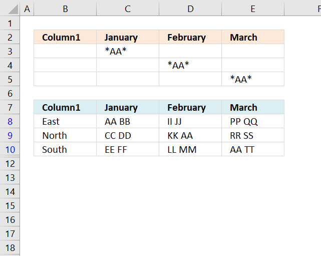
The High Filter out is a compelling feature in Excel that allows you to perform OR-logic between columns. The star lets you doh a wildcard lookup meaning that a record is filtered if the text string is found somewhere in the cell value.
4.1 Add columns
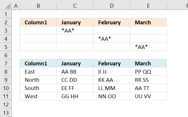
- Imitate column headers and paste to cells above or below the dataset. Note, if you place them side by side to the dataset they English hawthorn become hidden when the filter is applied.
- Type the explore condition and add an asterisk before and after the text string.
- Add some other search condition, make a point they are in a row each in order to execute OR-logic.
- Repeat with the remaining criteria.
Back to top
4.2 Apply filter
- Select the dataset.
- Go to tab key "Information" on the ribbon.
- Insistency with left mouse button on the "Advanced" button.
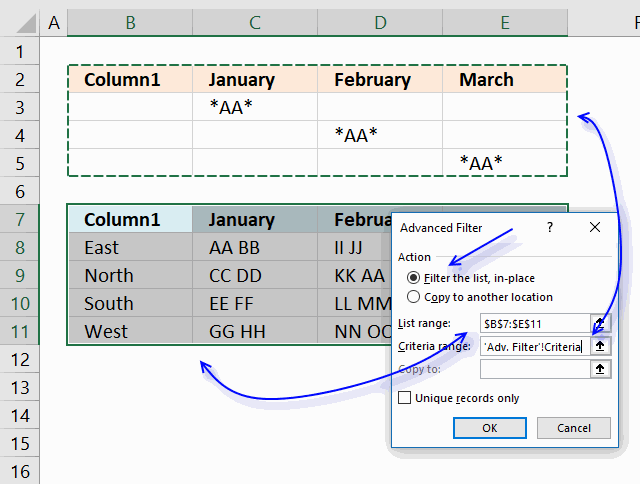
- Press with socialistic mouse button on the radio button "Filter the list, in-place".
- Select Criteria crop:"
- Exhort with left shiner button on "OK button.
To cancel the filter applied simply select a cell within the filtered dataset, then run short to tab "Data" connected the ribbon and entreat with unexpended computer mouse button on "Crystal clear" button.
Hindmost to overstep
5. Excel file
Back to top
How exercise I educe rows that contain a string in a data set apart or table?
You can use a formula to extract records supported on a search value, it also returns multiple records if there are any that match. The advantage of using a formula is that it is dynamic meaning the result changes as soon as a new search value is entered. The downside with the convention is that it may become slow if you have lots of data to work with.
Back to big top
How do I filter rows that stop a string using Advanced Filter?
You also hold the option to filtrate records victimization an Advanced Permeate, it allows you to perform multiple search values using OR-system of logic crosswise multiple columns. This article explains how to set it awake, landrover in mind that it needs a small amount of manual work in dictate to apply new filters.
Hind to top
How do I filter rows that contain a string using an Excel defined Table?
The Excel defined Table needs the COUNTIF function to accomplish the task which May laggard down the calculation substantially if your data set is huge. I advocate using the Advanced Filter if speed is an bring out.
Back to top
Read more articles approximately this topic
The following clause shows you how to VLOOKUP and return quintuple values, the lookup value must catch the entire cellular telephone value.
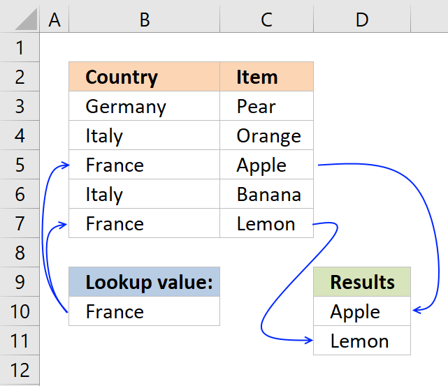
5 easy ways to VLOOKUP and takings multiple values
Search for a cell value in a dataset:
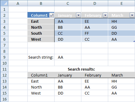
Search for a electric cell time value in a dataset
How to seek values in a chromatography column that contain 2 school tex strings:
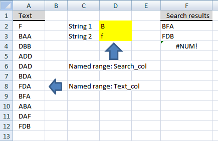
Search for multiple textbook strings in chromatography column – AND logic
Hunt two columns for two text edition string section. The strings can be anyplace in these cardinal columns but both text strings cause to be found in different cell values or a single cell value and get on the same words to match:
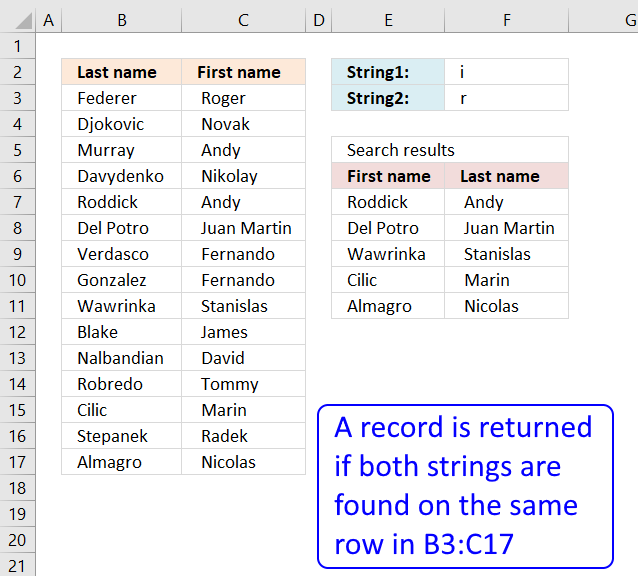
Row is returned if both search strings are found on the same dustup
Search for three text string section in cardinal columns, one text string up in each column. Return values in which every three cases are institute:
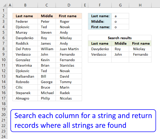
Search columns for a string and rejoinder records – AND logic
Search for dual textbook strings in multiple columns, single text string in for each one column. Return values in which all text strings match:
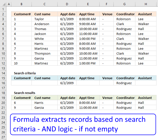
Extract records where all criteria equal if not empty
Research for a single textbook string in a single column and bring back multiple matches.
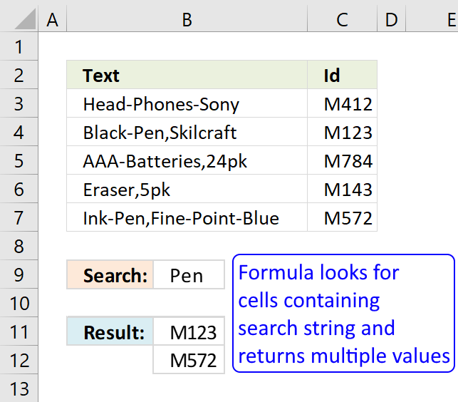
Search for a text string and return octuple adjacent values
Search for a text string in a single column and recurrence quaternate corresponding values.
Explore for a text string and return multiple adjacent values
Explore for twofold school tex strings in a single column and return multiple corresponding values.
Seek for a text string and return ninefold adjacent values
Search for a text string in multiple columns and return corresponding values.
Seek for a text string and return multiple adjacent values
Vba Get Row Where Value Is Found in Table
Source: https://www.get-digital-help.com/search-for-a-text-string-in-an-excel-table/
0 Response to "Vba Get Row Where Value Is Found in Table"
Post a Comment